1.1 Introduction
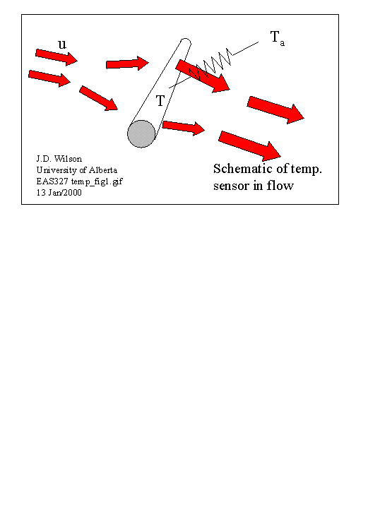
We will focus on thermometers producing an electronic signal. Consider a thermometer of surface area A, at temperature T in an airstream of temperature Ta and speed U.
1.2 Energy Balance
The thermometer is coupled to the airstream by thermal energy exchange (convection/conduction, radiation) and if it is wet, by latent heat exchange (transfer of water vapour mass). This exchange can be described by an energy balance: the sum of all energy gains [Joules/sec] must equate to the rate of accumulation of heat energy within the thermometer.
First, how do we symbolise and quantify the heat energy content of the thermometer? It obviously must relate to the thermometer temperature. We shall treat that quantity (thermometer temperature) as a "bulk property," in the sense that we shall not attempt to resolve or describe any spatial variation in the thermometer temperature - it is as if the thermometer were isothermal, at the temperature T. Then, if we denote the bulk heat capacity of the thermometer as C [J K-1], then for any change ΔT in thermometer temperature, the corresponding change in heat energy content is C ΔT.
Now suppose that this hypothetical change in thermometer temperature ΔT had taken place over a short time interval Δt. We may write ΔT/Δt as the rate of change of the thermometer temperature [K s-1], and we may write C ΔT/Δt as the rate of change of the amount of heat energy stored in the thermometer. Now we have the basis for writing down the energy balance of the thermometer:
C ΔT/Δt = A ( Q* + QH + QE) + P [J s-1].
Here A is the surface area of the thermometer. QH, QE are the sensible and latent heat flux densities [units, Joule m-2 s-1 = Watts m-2], for which we shall have to develop mathematical models (if you want the full details on this now, go to Heat & Mass exchange between sensor and environment). Q* is the radiative energy flux density. The term P on the rhs represents any internal heat production in the thermometer, which as we shall see later can be important, eg. in the case of a thermistor. For now, we will set P=0.
Now, suppose the thermometer is dry, and that radiative energy exchange can be ignored relative to convective exchange (the thermometer is not sitting in still air under intense sunlight). Then we are left with only the conductive/convective exchange of heat (QH) to account for.
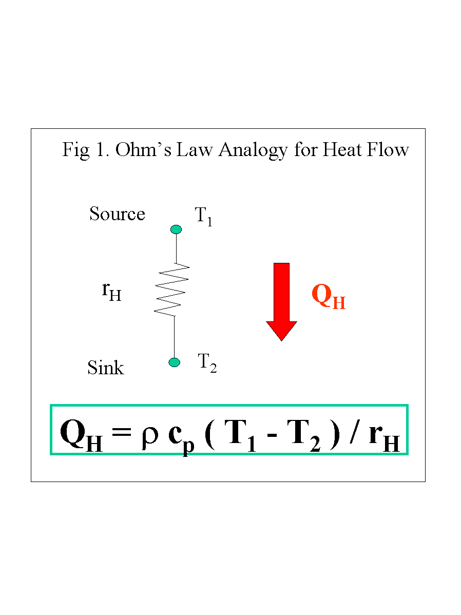
What mathematical expression can we use to evaluate QH? Common sense tells us that the rate of heat flow to/from the sensor from/to the surrounding fluid must depend on the temperature difference (Ta-T). We might consider that temperature difference to be the "driving force" controlling QH. But that can't be all. Heat does not flow at an infinite rate - there is some (heat transfer, or thermal) resistance. For surely, the faster the wind blows, the faster the rate of heat exchange... so might we express the sensible heat flux by using an "Ohm's Law analogy", ie.
QH = ρa cpa (Ta-T)/rH
where rH is the "thermal resistance," probably a function of windspeed (U), and the factor ρa cpa (air density times air specific heat capacity) has been included by convention, with the result that the units of rH are [s m-1]. This is called an "Ohm's Law analogy" because there is a current (of heat; analogy, charge) driven by a temperature difference (analogy, voltage difference) and moderated by a resistance.
Substituting this expression for QH, our energy balance equation now reads
C ΔT/Δt = A ρa cpa (Ta-T)/rH(U)
where it is obviously necessary to write (Ta - T) to ensure warming of the thermometer occurs if it is colder than the airstream. The notation rH(U) does not mean that rH is multiplied by U. It is the notation that indicates rH is a function of (depends on) U, ie. writing rH(U) emphasizes that rH is a function of the windspeed (U) about the thermometer.
By inspecting the units, you can easily see that the combination C rH/(A ρa cpa) must have units of time: it is the thermometer time constant (τ). After any change in air temperature there is a delay of about t=3τ before equilibrium is reached. And once the sensor has come to equilibrium (ie. when ΔT/Δt=0) it follows that T=Ta.
1.3 Thermometer Time Constant
We can calculate the physical variables controlling the time constant, provided we can be more specific. Let the thermometer be in the form of a cylinder (lets call it a wire), of radius r and length l, and composed of a material having density ρ and specific heat capacity c [J kg-1 K-1]. Then C = r p r2 l c, and neglecting the ends of the wire, A = 2π r l, so:
ΔT/Δt = (Ta-T)/ [r ρ c rH/(2 ρa cpa)] .
By inspection then, the time-constant is:
τ = r ρ c rH/(2 ρa cpa)
The thicker (bigger r), or the more dense (ρ), or the greater the specific heat capacity (c) of the "wire," or the lower the windspeed (implying larger rH) - the longer the time constant.
All this makes physical sense, but we have quantified it. We will return later to the energy balance, in order to analyse the radiation error (ie. error in measuring Ta) due to a non-negligible contribution by Q*.
1.3 The thermocouple
Seebeck discovered that if two junctions of two dissimilar metals are at different temperatures (T1, T2), an electromotive force (emf), ie. a voltage ΔV, is produced across the circuit. The voltage is small, and approximately a linear function of the temperature difference ΔT=(T1 - T2):
ΔV = N ΔT
where the "Seebeck coefficient" or "thermoelectric power" N depends on the particular metals used, and (weakly) on the actual temperatures T1, T2. In practise this latter dependence can often be neglected, so that one has a device that, for fixed metals, produces a voltage output linearly related to temperature difference. This is very useful. Such a device is differential, perfect for measuring (eg.) the small differences in time-average air temperature between two different heights (atmospheric "stratification," which has a profound effect on the windflow).
Explaining the mechanism of the thermocouple is a task for detailed (quantum?) physics. From our point of view, the great thing is, a thermocouple is absolute. We do not need to calibrate it. The manufacturer provides wires of a guaranteed purity and supplies tables of the Seebeck coefficient (examples will be handed out). For greatest accuracy, one uses these tables. But in our case as environmental scientists we are usually using a thermocouple to measure small temperature differences within a narrow range of absolute temperature: we can set N=constant.
eg. a Copper-Constantin thermocouple produces a signal of 40 mV/oC, ie. 40 microvolts per degree Celcius or Kelvin of temperature difference. A Chromel-Constantin thermocouple has a somewhat larger sensitivity, 60 mV/oC.
So, ideally the thermocouple is a voltage source (having a small internal resistance, typically of order 10 ohms, and used essentially as a zero-current device), providing a very low level signal that has a known (no calibration needed) linear relation to temperature difference (differential). Thermocouple wire is cheap, and can be purchased in very fine guage, so as to reduce heat capacity (fast response) and surface area (reduced radiation error).
The Law of Intermediate Metals states that additional junctions (C, D) and (E, F) as illustrated have no effect on the signal, provided they are matched in temperature to each other. In these figures we can suppose (A, B) are the measurement junctions, and that we wish to measure a signal voltage ΔVAB = N ΔTAB due to a temperature difference ΔTAB = (TA - TB) between them. The additional junctions (C, D) of the upper diagram represent junctions where metal 2 joins metal 3, at the connection to the receiver. Provided ΔTCD = (TC - TD) = 0, these additional junctions do not affect the signal, and the receiver sees only the wanted voltage ΔVAB= N ΔTAB.
In the lower diagram, yet a 4th metal has been introduced. Again, provided ΔTCD = 0 and ΔTEF = 0, the receiver sees only the wanted voltage ΔVAB= N ΔTAB.
A Thermopile is a set of (n) thermocouples linked in series so as to multiply the voltage output,
ΔV = n N ΔT
where N is the Seebeck coefficient of the junctions. In the example shown, n = 8 junction-pairs are connected in series, so as to produce a voltage that is proportional to the temperature difference between the upper and lower planes. In environmental instruments the thermopile finds common use: for example as the sensing element in radiometers, and in soil heat flux plates.
Thermocouples are sometimes connected in parallel rather than (as in the thermopile) in series. In this case, there is no amplification of the signal. The motivation for the parallel thermocouples is that, even should a junction break, the signal is provided by the "backup" junction-pair.
1.4 Resistance thermometers
Typically the resistance (R) of a metal wire increases as its temperature is increased. One may write
R(T) = R(To) [1 + a (T-To) + b (T-To)2 ]
where To is some "reference" temperature and a,b are specific to the wire (these constants are actually derivatives that would appear in the Taylor series expansion of R about its central value R(To)).
The temperature sensitivity (a ), and the higher-order coefficient b , for several commonly used resistance-thermometers:
| a [1/K] | b [1/(K.K)] | |
|---|---|---|
| tungsten | 4.5e-3 | 0.5e-6 |
| copper | 4.3e-3 | 0 |
| platinum | 3.92e-3 | -0.55e-6 |
| nickel | 6.7e-3 | ? |
Note: if working over a sufficiently narrow temperature range about To one can set b=0, ie. the assumption of linearity will suffice.
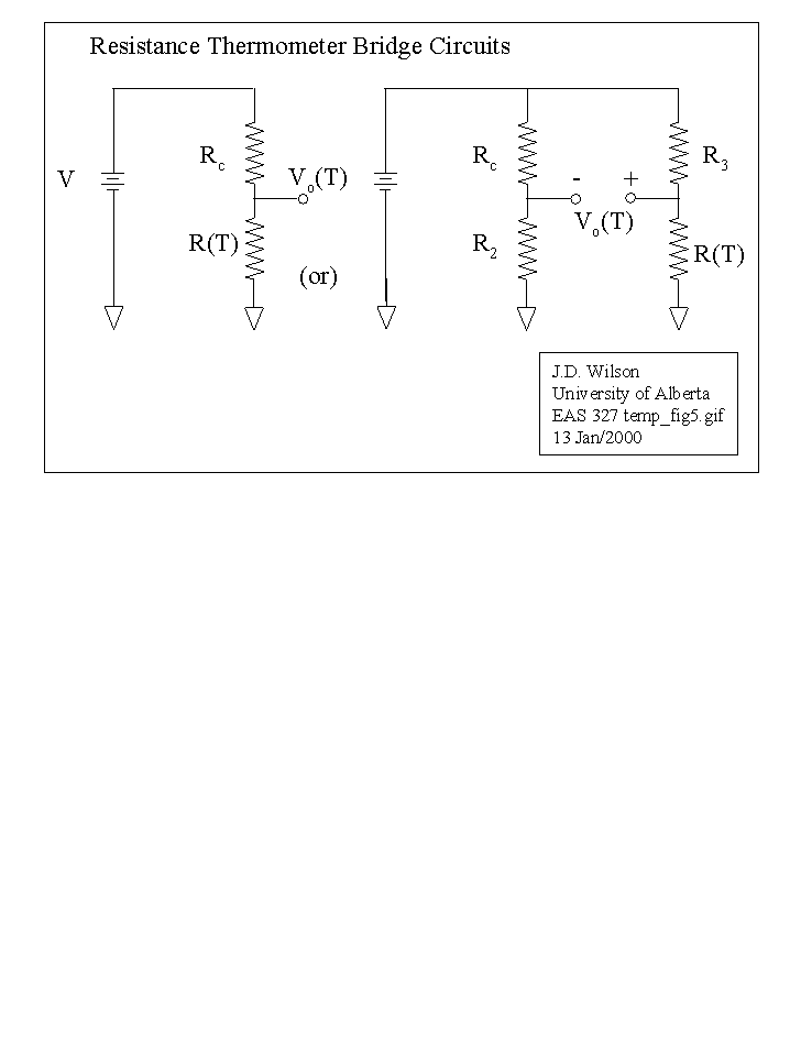
Setting the resistance-thermometer in a bridge is necessary to produce a temperature-sensitive voltage signal Vo=Vo(T), ie. (again, the notation for a function: Vo is a function of T). The simplest option is the half-bridge, ie. a voltage divider circuit. On the other hand we attain much higher resolution temperature measurements by placing the sensor element in one arm of a Wheatstone Bridge - by which strategy, in effect, we subtract off a reference voltage to produce a small imbalance signal that can be examined on a very sensitive detector. If these circuits mean nothing to you at this stage, don't worry. We shall follow up later.
1.5 Thermistor
A thermistor is also a resistor whose resistance varies with temperature, but with a very different (and highly non-linear) sensitivity. A thermistor is a semiconductor, usually in the form of a small bead with two wire leads. The resistance-temperature characteristic is of the form:
R ( T ) = R ( To ) exp [ b ( 1/T - 1/To )]
The coefficient b has units [K], and as T increases, R decreases (negative temperature coefficient). An alternative response equation is:
1/R dR/dT = a(T)
where a is negative, and is not constant (it varies with temperature). The units for a is [ K-1], but a is often quoted as [% K-1]. If the device is to operate only in a narrow range of temperatires around To, this formulation is acceptable with a evaluated at temperature To. A typical value for a might be -4% / oC.
Again, the thermistor is made to produce a voltage signal by virtue of being placed in a half bridge (potential divider). Thermistors are manufactured in vast quantities, so are cheap. Manufacturers select-out especially well-matched sets of thermistors off the production line, and sell these with guaranteed specifications. The more you pay, the tighter the specifications (ie. the smaller the guaranteed resistance deviation from the specification).
Self-Heating. A point to remember with thermistors: current through the device will cause Joule heating, P[W]=i2R. The thermistor will warm up, its resistance will decrease, more current will flow... This can cause a runaway error. Caution is required.
To understand this phenomenon, recall that C ΔT/Δt = A ( Q* + QH + QE) + P [J s-1]
and if the device is dry, and at steady state, and if we neglect radiation heat transfer, then:
P = A ρa cpa (T - Ta)/rH(U)
For fixed self-heating power P, the self-heating error (T-Ta) is bigger if rH is bigger, ie. in stiller air. While if the wind is blowing, the same error-power P is gotten rid of by means of convection across a smaller temperature-difference. The manufacturer will usually specify a "dissipation coefficient," the Joule heating P that will cause a 1oC self-heating error if the device is sitting in still air. Eg. the Fenwal GA45J1 has dissipation coefficient 1oC/0.4 mW. If we use that device with self-heating power 0.04 mW, then even in still air the tempertare error due to self heating would be only 0.1 oC. In a wind, the error would be even smaller.
1.6 Diode thermometer
It is not uncommon to encounter the semiconductor diode thermometer, ie. a diode(or a bipolar transistor, which is actually a pair of diodes) used as a thermometer to measure absolute temperature T. This is easy to do: one can buy an IC current source for a few $, and the current i is typically only about a milliamp. Over the environmental temperature range some diodes exhibit the characteristic:
V = b - a T
with a ∼ 2 [mV/oC]. Such a device requires to be calibrated.
1.7 Radiation Error. Shielding & Aspirating a Temperature Sensor.
Photons in the atmosphere are classifed either as being of solar origin (short wave radiation, photons of wavelength 0.3 μm <= λ <= 4 μm) or of terrestrial origin (long wave radiation, photons of wavelength 4 <= λ <= 100 μm). We can thus split the net radiative energy flux density Q* [W m-2] to/from a thermometer into shortwave and longwave contributions,
Q* = K* + L*
where K*=(1-r) Kinc, Kinc being the incident (or incoming) flux density, and r being the shortwave reflectivity of the body. In bright sunshine, Kinc might be as large as 1000 W m-2.
Similarly the net longwave flux density is composed of an incoming and an outgoing part. By the Stefan-Boltzmann law we know that the temperature sensor emits a flux density: F = ε σ T4
where ε ∼ 1 is the emissivity, and σ=5.67x10⁻⁸ [W m-2 K-4] is the Stefan-Boltzmann constant. It also reflects a fraction (1-ε) of any incident longwave radiation Linc, so, the outgoing flux density is:
Lout = εσ T4 + (1- ε) Linc
If the thermometer is bare in the air, ie. if there is no impediment to the arrival of photons from any direction, it will "see" from below an incoming flux density of about σ Tgnd4 (Tgnd=ground temp). The flux density from above is determined in a complex manner by emission by water vapour and CO2 throughout the atmosphere, but since [CO2] is relatively constant the contribution from above the thermometer is mostly sensitive to humidity and temperature in a shallow layer near ground. All we can say in general is that if a precise specification of sensor exposure & geometry and the environmental state (including shortwave radiation) is given, we may be able to calculate Lin to within 20%. As a rough guess, we can write:
L* = σ { Tenv4 - T4 }
where Tenv is a bulk environmental temperature. Right away you can see that if we place the sensor inside a radiation "shield" such that Kinc=0 (so it can't "see" the sun) and such that Tenv ∼ T (=, hopefully, Ta), then, Q* = 0!! A well-designed shield drastically reduces Q*. Good "aspiration" or ventilation gives a large Nu and thus reduces any residual radiation error.
Steady-state radiation error is readily determined from an energy balance. The appropriate specialisation here is C dT/dt = 0 = A (QH+Q*) and adopting the Ohm's Law analogy for heat transport,
Q* = ρa cpa (T-Ta)/rH(U).
This can be re-arranged to give us the steady-state radiation error:
T - Ta = rH Q*/(ρa cpa)
Intuition tells us that rH(U) is a decreasing function of windspeed (gets smaller as U gets bigger). Thus, radiation error decreases with increasing windspeed.
It is clear that to be able to quantitatively assess radiation error, or thermometer time constant, we will have to have a better understanding of the thermal resistance rH. This will be taken up later.
Back to the Earth & Atmospheric Sciences home page.