- Tues 9 April. Weather briefing (Tobe and Chris). Review/questions.
- Thurs 4 April. Weather briefing (Jean-Michel and Brett). NWP, continued.
- Tues 2 April. Weather briefing (Darren and Danielle). NWP -- Canada's GEM model. (Optional further reading: a primer on initialization of NWP models).
- Thurs 28 Mar. Weather briefing (Allen and Ambrose). Using the Monin-Obukhov temperature profile to "calibrate" the bulk model for QH. Energetics of snowpack: covering the many factors controlling the duration of time before sufficient energy accumulates to melt the existing snow cover (whose depth is given by the Environment Cda. analysis as currently 30 cm of more). Time permitting, some work on tasks (2,3,4) listed Thurs 14 March. Please complete these as homework.
- Tues 26 Mar. Weather briefing (Jennifer and Tara). Discussion of last Thursday's snow storm (below). Continuation of exercises using GrADS.
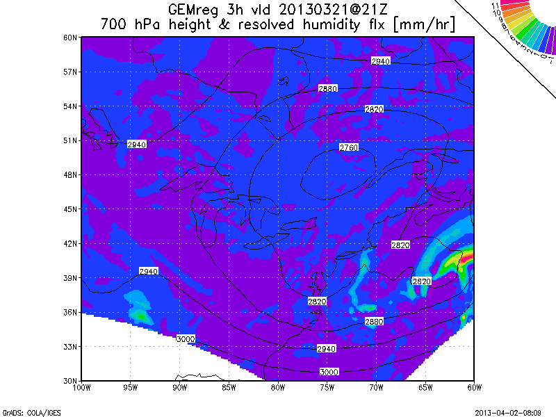
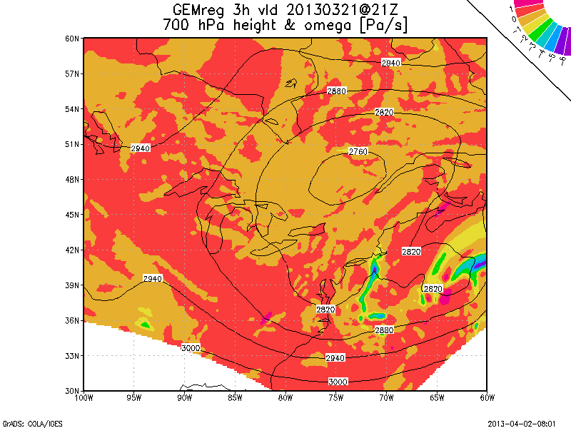
- following the steps documented at GrADS, download the .grib2 files needed to plot the resolved vertical flux of water vapour at the 700 hPa level, based on GEM prog (choose whatever time looks interesting)
- Note that the vertical vapour flux can be written: E = ρ q w, where q is the specific humidity. It appears on first sight that you will need to define the density field (as in last week's exercise), however given that w=-ω/ρg we can also write E = -ω q / g. Thus computing the density is not essential.
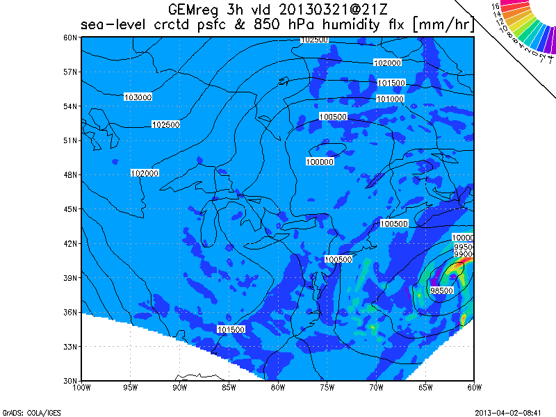
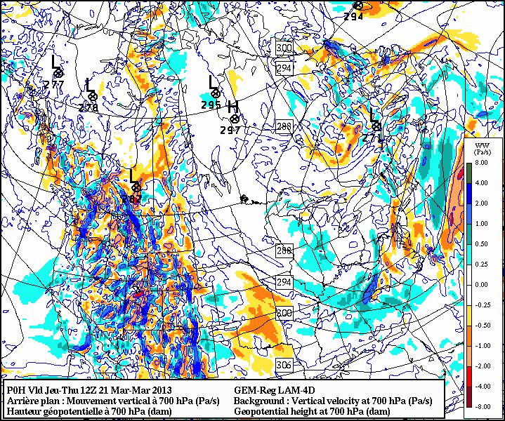
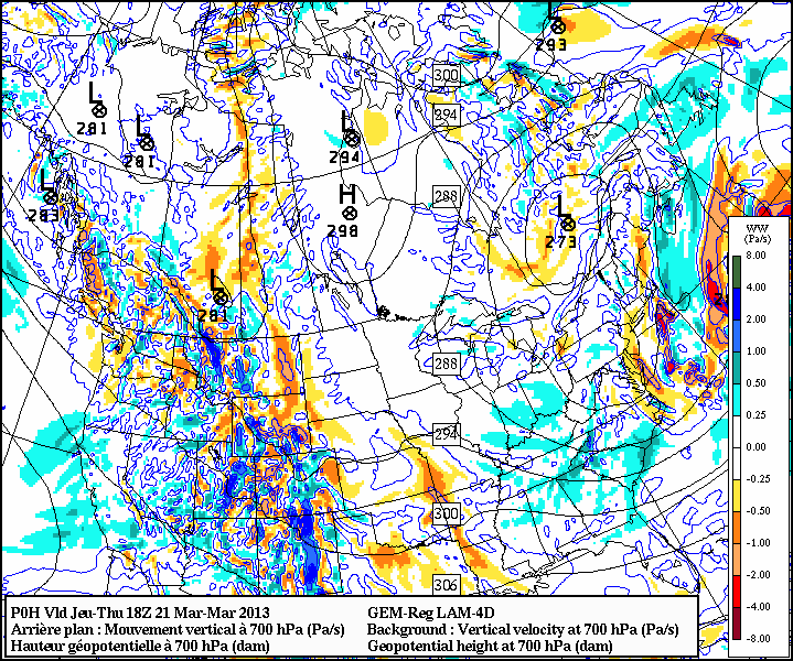
Please hand in such a plot (example: resolved humidity flux at 700 hPa level, 21Z March 21; the associated 700 hPa omega field; the corresponding humidity flux at 850 hPa, and surface isobars. Notice how the "comma pattern" shows up in the humdity flux). What snowfall rate in mm/hour corresponds to your maximum flux (assuming 10:1 for the ratio of snow depth to liquid depth)?
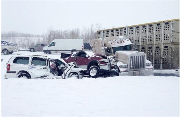
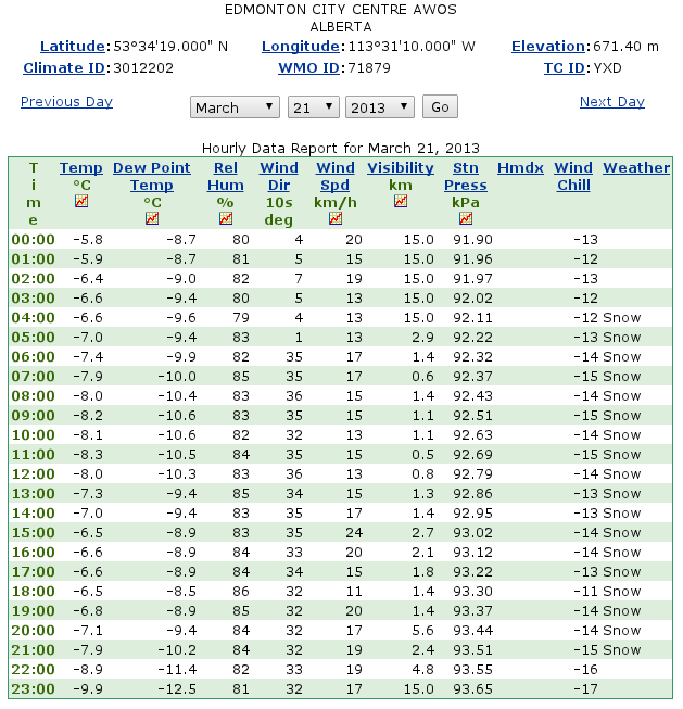
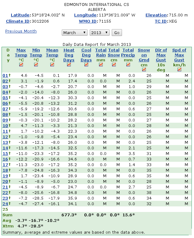
- According to David Phillips of EC, we've had continous snow cover since 10 November 2012. The snowstorm of 21 March dropped us another 20 cm or so around the city. The rate of snowfall was high at times and places. Accumulations were rather non-uniform (Edmonton city, hourly and YEG daily records). Over 40 cm of snow accumulated, reportedly (though this is word-of-mouth and remains to be confirmed), at Westlock.
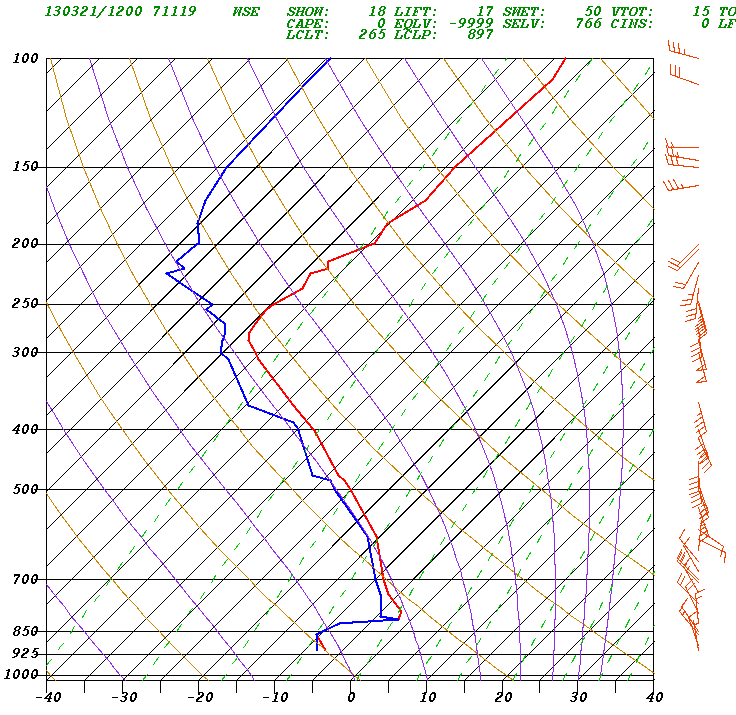
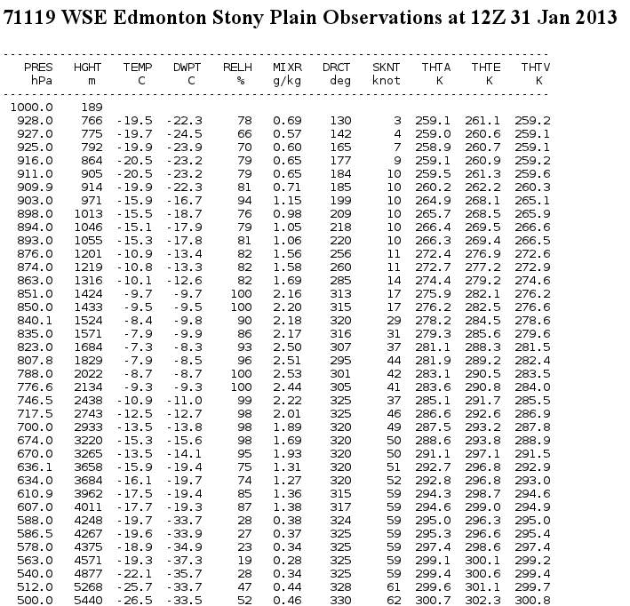
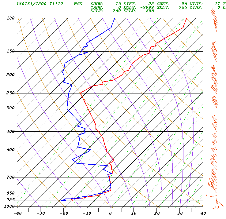
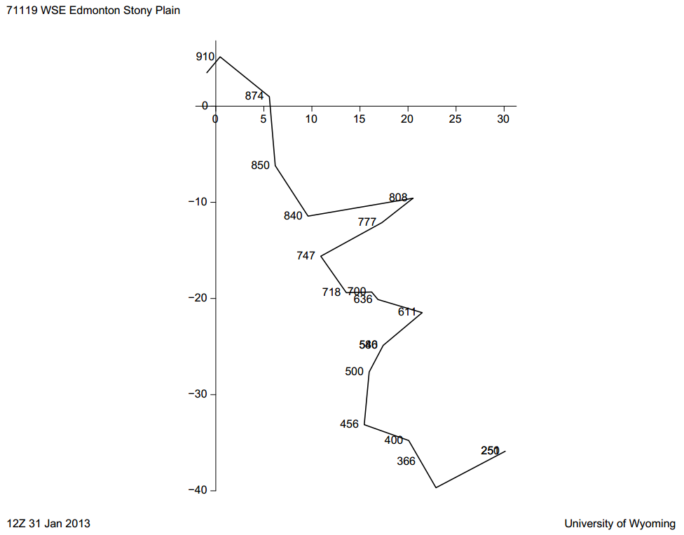
- the 12Z Edmonton sounding shows a cold stable saturated layer overlain by a deep, neutrally-stratified layer. The stable layer is incapable of generating heavy snowfall, because vertical motion is strongly suppressed. Conversely, there is no impediment to vertical motion in the deep neutral layer, which must (therefore) have been the generator of the heavy snowfall rate. That deep vertical motion was occurring is indirectly verified by the fact that cloud-cloud lightning was observed. (Notice too, the directional wind shear between 600 and 550 hPa).
- the 12Z surface analysis shows a trough through Alberta and a ridge through Manitoba, with strong pressure gradient across Saskatchewan. There is a closed low in S. Alberta, and central Alberta is experiencing an easterly, upslope outflow from the ridge to our east. There is temperature contrast, but it isn't that dramatic. By 18Z the low has moved eastward, and by 00Z (Friday) it straddles the border. Thus the low is not a fast-mover.
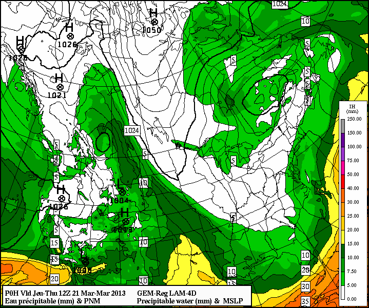
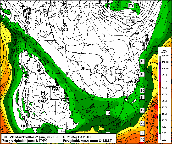
- precipitable water as of 12Z. The 10-15 mm over Edmonton, if converted to snow with a 10:1 snow/water depth equivalence, would produce 10-15 cm of snow.
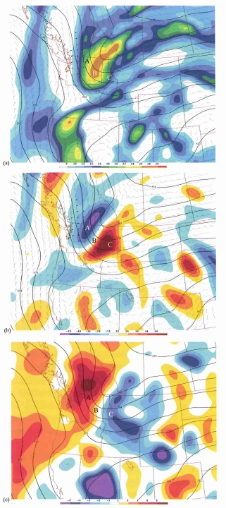
- at 500 hPa we see a southerly flow over Edmonton exiting from a trough. The 500 hPa height/vorticity chart (cropped from the b/w 4panel chart for the GEM reg 0h prog) implies PVA over south-central Alberta --- significant for height falls and ascending vertical motion
- at 12Z at the 700 hPa level we see a supply of moisture, and the GEM reg 0h progs indicate lift (12Z) and at 18Z
- at 12Z at the 850 hPa level we can safely surmise zones of thermal advection in the region of the low: cold advection over south-central Alberta (somewhat counteracting the effect of the PVA in the omega equation) and warm advection over southeast Alberta (where it will complement the effect of PVA in the omega equation) and southwest Saskatchewan
- Dr. Reuter points out that in the deep neutral layer, where the static stability parameter σ=0, PVA can have the effect of pulling up the whole layer (it is interesting to note that 1/σ multiplies several terms in the QG-omega equation, amplifying such terms as σ gets small).
- Thus 21 Mar. The atmospheric surface layer (constant flux layer). The friction velocity. The turbulent temperature scale. The Monin-Obhukov theory of the surface layer. Interpretation of the Obukhov length. The log wind profile. Bulk model for the sensible heat flux QH. Exercises:
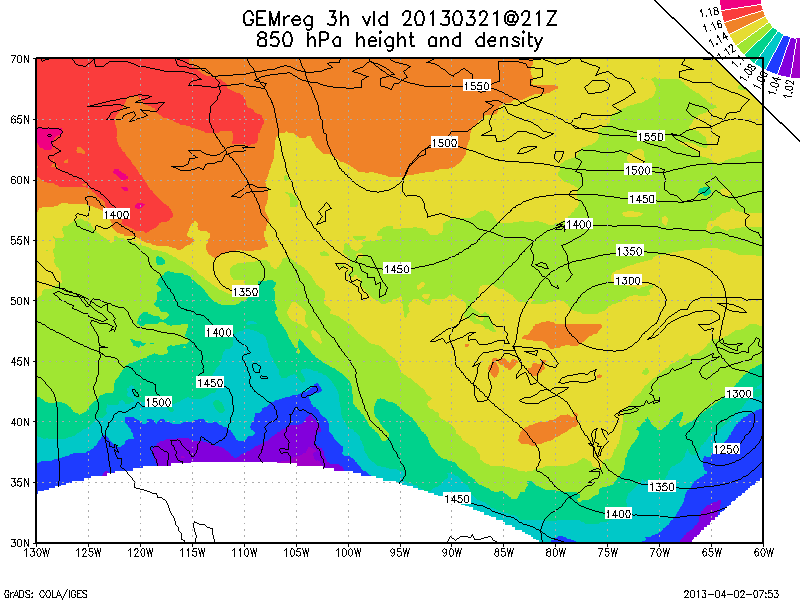
- using GrADS, compute and plot the field of air density at 850 hPa level from a GEM reg field of temperature. Download the .grib2 file for the 850 hPa temperature. Following the steps outlined in file GrADS, set up an XWin Server terminal and:
- g2ctl filename.grib2 > filename.ctl
- gribmap -i filename.ctl
- now open GrADS in your terminal (type "grads"), and within grads
- open filename.ctl
- set lat 30 70
- set lon 260E 320E
- q ctlinfo [this will tell you the names of the variables available to be plotted]
- define rho=85000.0/(287.0*tmp850mb)
- display rho
- the above gave you a contour plot (the point of which exercise is to show how easily we may use GrADS to compute and display derived fields; but notice, too, the inhomogeneity of the density field - any fronts about?)
- clear the display (issue "c" or "clear"). Then "set gxout shaded" and again issue "display rho"
- this is fine, but what is the colour code? At this point, exit GrADS and download cbarc.gs your directory in cgwin, i.e. to c:\cygwin\home\yourccid
- re-enter grads, again compute the density field and display it as a shaded map. Now issue "cbarc". This should provide a scale
- draw title GEM reg ??h forecast valid 201303??@??Z\air density at 850 hPa level
- printim mygraph.png png white
- please save your graph to a permanent spot and print it off to hand in
Here is an example based on the .grib2 fields from a 3h GEM reg prog valid 21Z March 21 (note: here I used the "cat" command to concatenate the .grib2 files for 850 hPa height and temperature before creating the .ctl file, so as to be able to also plot the height contours). When you are satisfied you have understood and completed the above, please move on to exercises 2,3,4 given 14 March.
- Tues 19 Mar. Weather briefing (Toby and Chris). Went over the exercise (nominally, begun 5 March) relating to Lackmann's Figure 2.7, PVA and vertical motion downwind of an upper trough, and (relating to Lackmann's Figure 2.8), over veering and backing of the wind in relation to temperature advection. Intro. to GrADS: we plotted a single field from today's 00Z GEM glbl run.
- Thurs 14 Mar. Weather briefing (Allen and Ambrose). Exercises (for today and into next week):
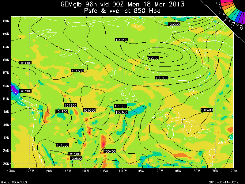
- Following the information given in this file concerning GrADS, download the following .grib2 files from (today's) 00Z GEM global run and valid 00Z Monday 18 March (96 hr prog):
- sea-level corrected surface pressure, CMC_glb_PRMSL_MSL_0_latlon.225x.225_2013031400_P096.grib2
- vertical velocity ω at 850 hPa, CMC_glb_VVEL_ISBL_850_latlon.225x.225_2013031400_P096.grib2
Use GrADS to display these two fields, focusing on the storm at the southern border of Manitoba. (You should get something like this).
- Use Lackmann's Eq.(1.58) in an approximate form (assuming horizontal homogeneity and that the diabatic term J=0) to estimate the surface heat flux QH0 [W m-2] on a morning when the temperature increased by 3K from 11 am to 12 am, and the mean depth of the ABL was 800 m. (Method: approximate the eddy heat flux divergence as a finite difference between QH=0 at z=800 m and QH0 at ground.)
Answer: QH0 ≈ 670 W m-2
- If the temperature in a horizontally-homogeneous surface layer is increasing at 1 K hr-1, what is the difference between the heat flux at ground (QH0) and the heat flux (QH) at z=10 m?
Answer: ΔQH ≈ -3 W m-2
- Compute the mean rate of heat loss to ground QH0 [W m-2] corresponding to the observed overnight cooling at Edmonton between 00Z and 12Z on 13 February, 2011 (I ought to have specified: consider only the layer below 4 km, neglecting changes further aloft, which were probably caused by thermal advection). Obtain the underlying data and plot T versus height z for each sounding (on the same graph ). The area enclosed by the two soundings, multiplied by an approximate value for ρ cp, is the energy lost over the twelve hour interval. Note that a unit of area on your T versus z graph has dimension [K m].
Answer: computed energy loss to ground. The area on your graph will be (say) "X" [K m] and can also be written X [K m3 m-2]. Now, a change of 1 K in the temperature of X m3 of air consumes or liberates an amount of energy equal to ρ cp X [J]. Therefore the area on your graph corresponds to the loss of ρ cp X [J m-2] over 12 hours. Then the effective surface heat flux is QH0 = - ρ cp X /(12 x 3600) [W m-2].
- Tues 12 Mar. Weather briefing (Darren and Danielle). Micrometeorology (continued): rules for (Reynolds) averaging; water vapour budget in a horizontally-uniform atmosphere. Simplified form of the continuity equation in the ABL (div u=0), and implied mean vertical velocity in a horizontally-homogeneous ABL. Significance of the vertical eddy flux. Continuation/completion of exercise begun 5 March. GrADS image of 850 hPa height and vert. veloc. for the Toronto storm.
- Thurs 7 Mar. Weather briefing (Jennifer and Tara). Basics of micrometeorology for treatment of processes in the ABL (friction layer): convention for averaging ("Reynolds averaging"); physical mechanism of, and notation for, the eddy flux (also known as the "turbulent" or "unresolved" flux) of sensible heat (and other eddy fluxes). Influence of eddy fluxes on the evolution of the "resolved" (or average) properties (Lackmann's Eq. 1.58). Continuation of exercise begun 5 March.
- Tues 5 Mar. Weather briefing (Jean-Michel and Brett). Significance of "solenoids" on the cross-section associated with this cold front (00Z, 1 Jan. 2011), in relation to baroclinicity and geostrophic advection of temperature (continued): we prove that in a barotropic region of the atmosphere, there are no solenoids.
Exercises (for today, and continuing Thurs 7 March):
- Completion of the cross-section(s) started 28 Feb.
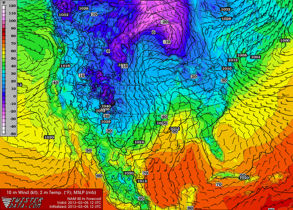
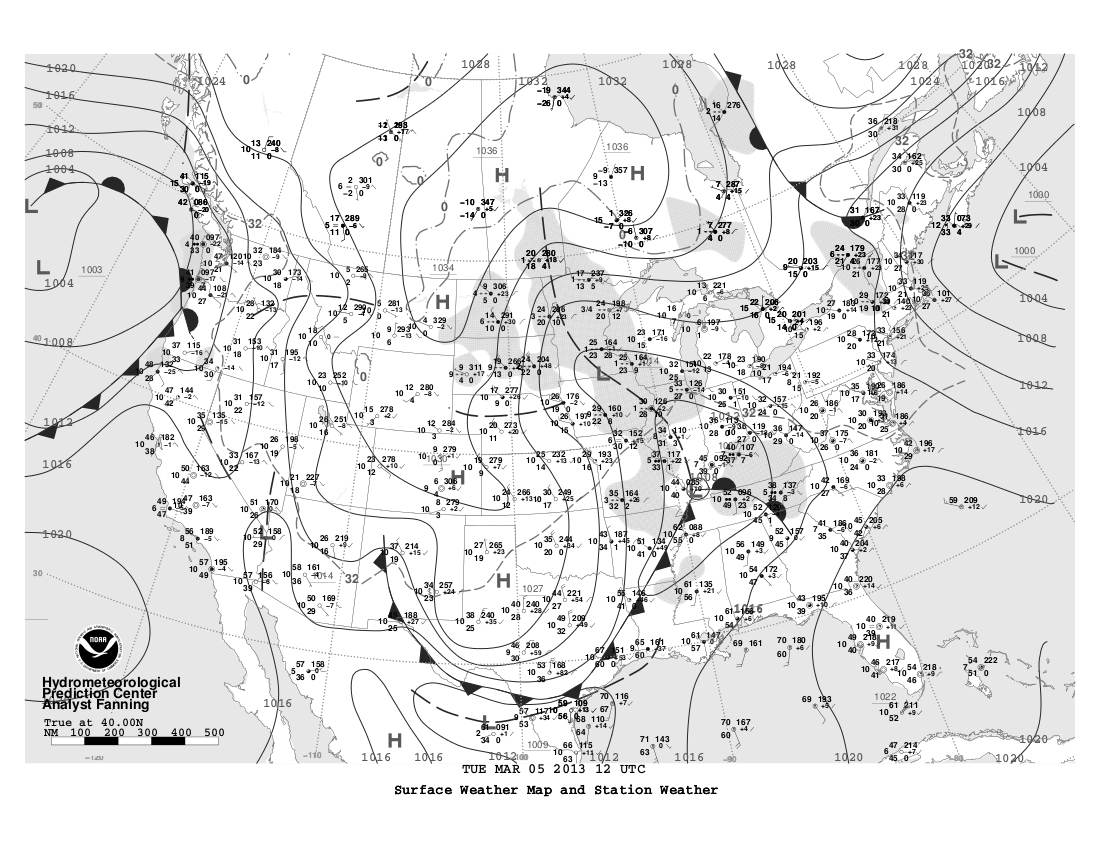
- Analyse fronts associated with the weather system in the SE United States (SE Missouri) on today's 12Z surface chart (12Z, 5 Mar. 2013, cropped). This analysis (full size) sourced at Meteocentre (=> Analyses => Surface - North America). Typically, bunching of isotherms at the 850 hPa level provides useful guidance for analysis of fronts (this chart, valid 12Z on 5 March 2012, is the 0-h GEMreg prog, and has been obtained by cropping the "Classic 4-panel Black & White Chart"). Many other charts are available that can help with deciding where to locate fronts, e.g. from Twisterdata.com here is a surface analysis including 2m temperature and winds. Please use the standard notation to indicate your fronts.
Answers: NOAA analyst's fronts, CMC analyst's fronts.
- Reproduce Lackmann's Figure (2.7a) for 500 hPa height and vorticity, from the Plymouth State Weather Center archive. Suggested settings:
- 2008 Sep 10 0Z (06Z is unavailable)
- Region: Northwest, Map Size: 1024 x 768
- Variable 1: Geopotential Height, Level: 500 mb, Contour/Plot Type: line , Interval: 60, Color: black
- Variable 2: Absolute vorticity, Level: 500 mb, Contour/Plot type: dashed line, Interval:4, Color: red
Please save and print your chart (in the lab, if you have print credits; or elsewhere) and submit, with a comment as to the meteorological significance of this height/vorticity pattern (covered by Lackmann, pp45-46).
Answers: Reconstructed Lackmann Figure 2.7a using lines only, and using color fill for absolute vorticity. Note: I have used 30 dam contour interval. To get a color fill plot, the field to be shaded must be Variable 1.
- Using the same resource, produce a shaded plot of the convergence at the 850, 700 and 500 hPa levels.
Answers: Convergence (and geopotential height) at the 500 hPa level, lines only, and using color fill. Likewise, convergence at the 700 hPa and 850 hPa levels.
- Lackmann's Figure (2.7c) gives the field of vetical motion (ω) at 500 hPa. Using the resource at NOAA, produce charts for ω at the 500, 700 and 850 hPa levels.
- Variables: Omega, Analysis levels: 500
- Sep 10 6Z to Sep 10 6Z 2008
- Color Shaded
- Scale Plot Size 200%
Please save and print your chart, and submit with a comment as to the meteorological significance of this vertical motion pattern (compare your chart for ω at 500 hPa with Lackmann's Figure 2.7c).
Answers: Vertical motion field at the 500 hPa, 700 hPa and 850 hPa levels.
- Another Plymouth State Weather Center link allows us to access the NCEP/NCAR Reanalysis Upper Air Maps. Focusing now Lackmann's Figure (2.7) pertaining to an upper trough over Washington State at 06Z on 10 September 2008, use this resource to produce a chart of vorticity advection at the 500 hPa level and compare with Lackmann's Figure (2.7b). Suggested settings:
- Northwest 500 mb Vorticity advection 0.5 color fill 2008 Sep 10 0Z
- Overlay this field 500 mb Geopotential height 30 line 2008 Sep 10 0Z
Answers: NCAR Reanalysis for the field of vorticity advection at 500 hPa at 00Z on 10 Sept. 2008 (c.f. Lackmann's Figure 2.7b).
See also file Lackmann_Fig2p7.pdf.
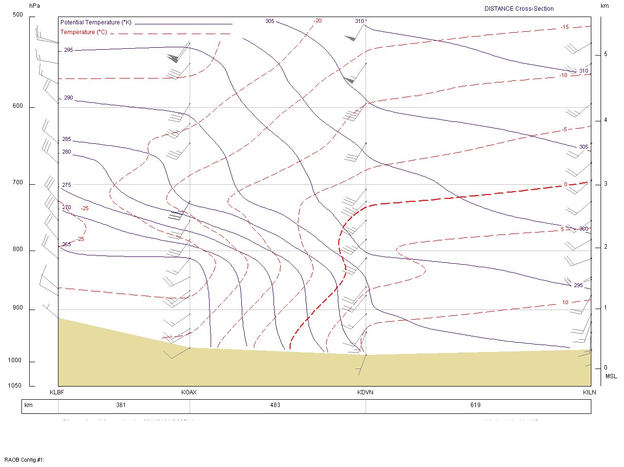
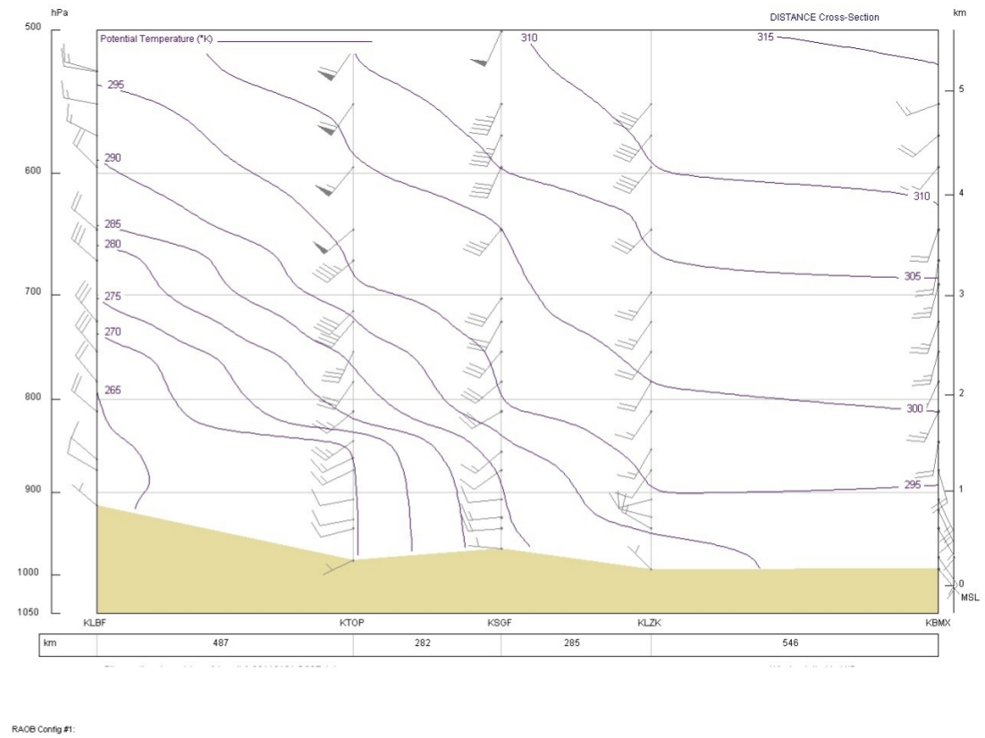
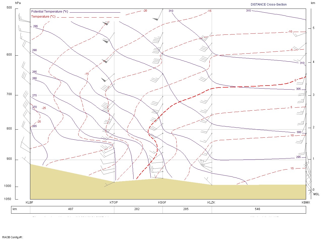
- Thurs 28 Feb. Weather briefing by JDW (note: the material on the storms in the eastern U.S. was not covered, for addressing the W. Canada situation and prognosis consumed about 25 min). Theory: understanding the significance of "solenoids" on the cross-section (intersections of isotherms and isentropes), in relation to baroclinicity and geostrophic advection of temperature: we proved that in a barotropic region of the atmosphere, geostrophic temperature advection vanishes. Exercise: plot isotherms for T=(-40,-35,-30,-25,-20,-15,-10,-5,0,+5)oC on this cross-section (hard-copy handout, with isentropes already plotted) from the radiosonde data (note: if this is not the cross-section for which you plotted isentropes in the previous class, you may instead add isotherms to your previous cross-section).
Answers. Please compare your cross-section(s) with those plotted by RAOB, for LBF to ILN and/or for LBF to BMX. These cross-sections (valid 00Z on 1 Jan. 2011) have both isentropes and isotherms plotted, and the solenoids correspond to regions of thermal advection. To estimate the static stability σ at ILN, many approaches could be taken (the instructions were not very specific). JDW took the difference between θ values of 305oC at 650 hPa and 295oC at 850 hPa. Then the difference Δln θ=0.033, and with Δ p=-2x10⁴Pa and ρ~1 then σ ~ +1.7x10⁻⁶Pa-2s-2. Holton (Dynamic Meteorology, 4th edn, p150) states that in the mid-troposphere typically σ~2.5x10⁻⁶.
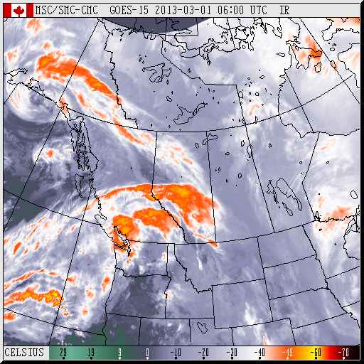
Follow-up on weather briefing. The GOES ir image (06Z Friday 1 March) shows the expected "dry slot" in the lee of the Rockies that is a common feature of the lee trough scenario (caused by sink). The 700 hPa analysis and the 850 hPa analysis are consistent with the progs shown in the briefing. Notice the warm air aloft in the lee of the mountains. (Note: this is not the ideal illustration of the Alberta lee trough, for in this case the 700 hPa contours indicate a geostrophic wind that must be obliquely incident on the mountains. That is, the 700 hPa height contours are not lined up perpendicular to the Rockies; and nor is the 700 hPa flow particularly strong.)
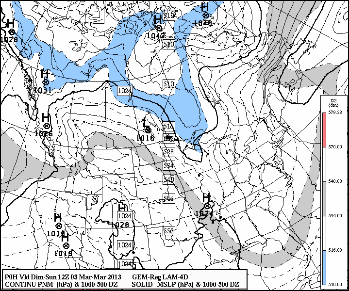
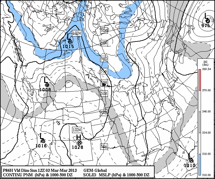
Here is the GEMreg 0h prog (12Z Sunday 3 Mar) for comparison with the 84-h forecast given in Thursday's briefing.
- Tues 26 Feb. Schedule student weather briefings (trial run & scored run). Clarifications regarding most recent exercise: terminology for station reports; decoding T and Td on surface and upper charts; distinction between sea-level corrected and true (station) pressure. Coming weather? -- 336-h GFS forecast (valid 06Z Tues 12 March). [Added 5 March: latest, and much shorter-range, 162-h GFS forecast for the same valid time. There are many qualitative similarities between these two progs. Added 11 March: NAM 18-h prog valid for same time].
Today's exercises will use radiosonde data in this file:
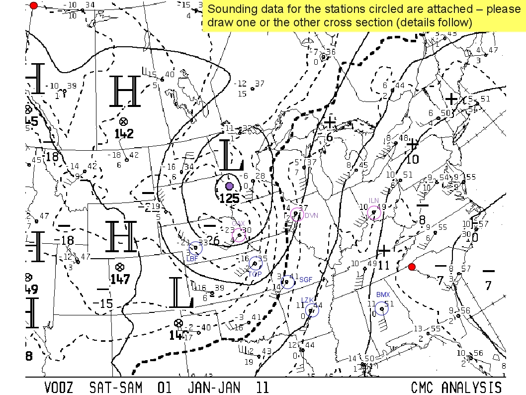
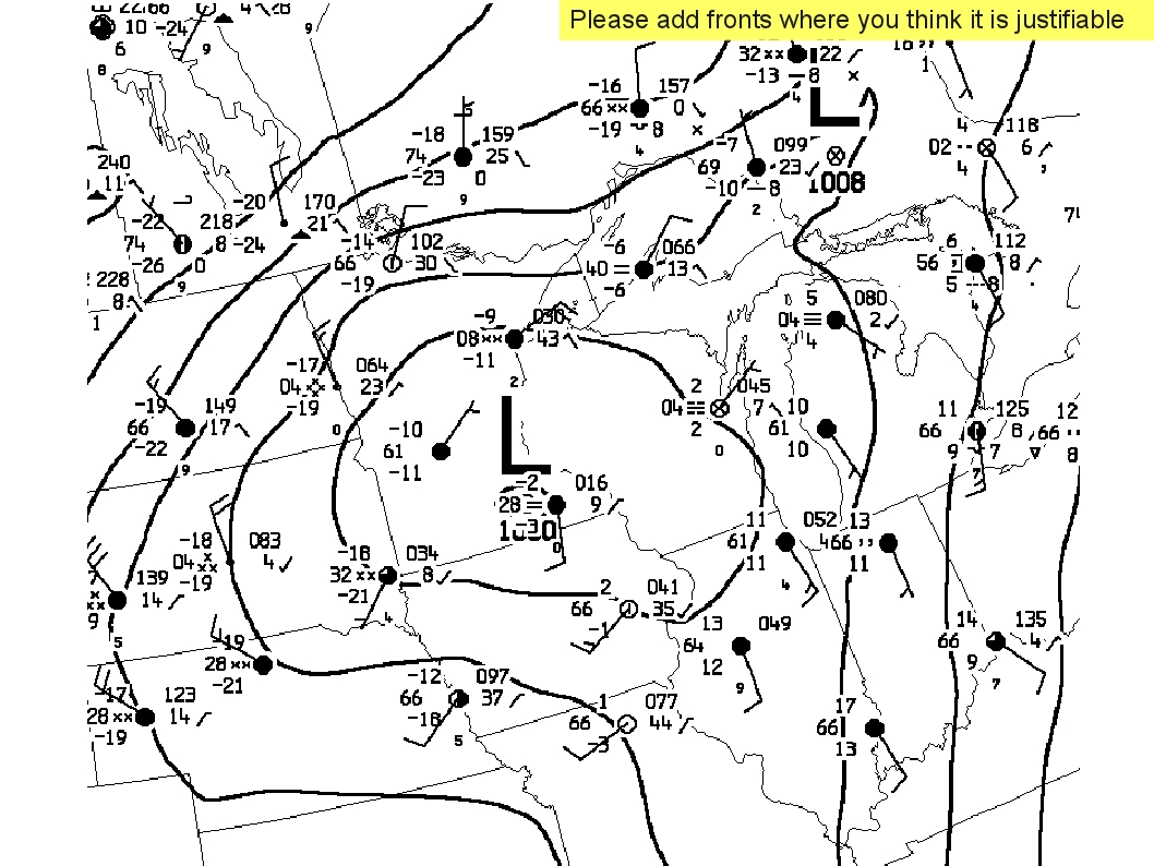
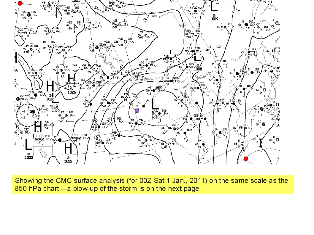
- add fronts to the CMC preliminary surface chart for 00Z, 1 Jan. 2011 (here is the same chart, with wider coverage). The isotherms at 850 hPa give some guidance.
- plot a height-distance cross-section associated with this cold front (00Z, 1 Jan. 2011)
- calculate static stability (σ) at ILN (Wilmington). Identify "solenoids" on the cross-section, from orientation of grad-theta relative to grad-T
- Thurs 14 Feb. The Quasi-geostrophic model: assumptions; vorticity equation; omega equation. Follow-up on Tuesday's exercise: find the LCL and LFC, and shade in the area representing CAPE (convectively available potential energy), on this Stony Plain sounding (00Z, 8 August 2008).
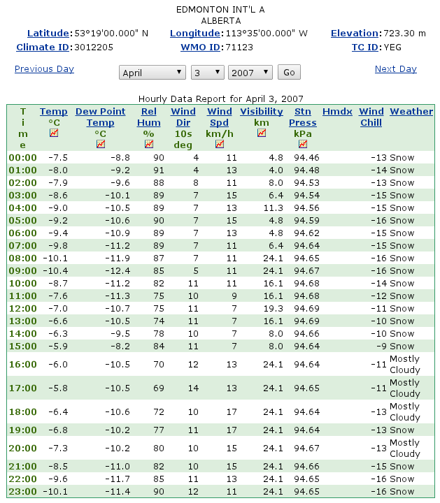
- Tues 12 Feb. Action of the Laplacian operator on a single "mode" (wave) T=T0 exp[j(k•x + ωt )] of the temperature field: by straightforward differentiation we proved that (in this special case) ∇2 T → - | k |2 T, where k is the wavenumber vector (and the arrow means "can be replaced by"). Exercises: Compute std. dev of a random variable x having (a) uniform distribution on [-1/2, 1/2] and (b) triangular distribution on [-1,1]. Find the LCL and LFC on this Stony Plain sounding (00Z, 3 April 2007). Cross-check the 850 hPa temperature and dewpoint with the 850 hPa analysis. Retrieve the hourly data for YEG on this day. What low cloud types are noted on the surface analysis at this time? What does the present weather symbol signify for the station in the NW corner of Alberta? Compute the surface air density at that station.
Answers: The variance of a variable having uniform distribution on [-1/2, 1/2] is 1/12, so the std. dev. is the square root of this; the variance of a variable having triangular distribution on [-1,1] is 1/6, so (again) the std. dev. is the square root of this (we did both examples in class). Hourly data for YEG (3 April 2007). Low cloud types reported (on the sfc analysis) in Alberta were Cu and SCu. Present weather for the station in the NW corner of Alberta was blowing snow (see wxchart.pdf). Surface air density there was ρ=P/Rd T = P/(287 x (273.15-11))= . But what was P? We need the true (station) pressure, but the station report gives us sea-level corrected pressure (which was 1041.5 hPa). There is no readily available archive we can turn to to get the true pressure: as a first approximation, if we knew the height Δz of the station above sea level we could subtract ρ g Δz (but we'd have to guess ρ!).
- Thurs 7 Feb. Finite difference representation of the Laplacian operator (demonstrated for a heat equation in two space dimensions). Probability density functions (PDFs): orientation to Assignment 3. Homework for next class: determine the standard deviation of a variable x that is uniformly distributed on [-1/2, 1/2].
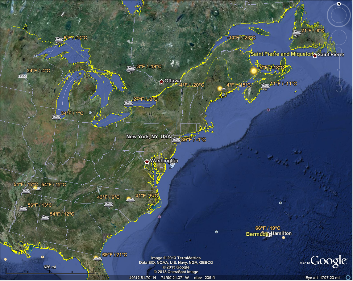
Exercise (please submit today): describe the cloud pattern offshore on the east coast (New York region) on the latest GOES east visible image. In a few paragraphs, give your brief qualitative forecast for central Alberta centred around 18Z Saturday 9 Feb; and for New York 00Z-12Z this Saturday 9 Feb (i.e. mid Friday through Saturday morning).
Here are (some of) the available NWP charts, along with follow-up (verification).
- Tues 5 Feb. Hand back exercises, and Assignment 1. Question period -- opportunity to clear up points of confusion (e.g. meaning of the 540-534 dam thickness band; whatever else may be perplexing anyone). Exercise catch-up time. Derivation of the heat equation (heat conservation in presence of conduction, convection, radiation and local production).
- Thurs 31 Jan. Continuity equation in the isobaric coordinate system. Relationship between omega and ordinary vertical velocity w. Exercises: plot a hodograph for today's 12Z Stony Plain sounding (here's the skew-T diagram). Identify (draw on your hodograph) the thermal wind VT,700-850, and comment on the relationship between your thermal wind vector and the isotherm pattern at the 850 hPa and 700 hPa levels. (Note: 1 m s-1 = 1.94 ≈ 2 knots.) Identify on the 12Z surface analysis the highest (largest) rate of change of surface pressure (Pa s-1) occurring on the Canadian prairies (enumerated as the pressure change, in tenths of one hPa, in past 3 hrs). Using the omega-w relationship, compute the implied value of the vertical velocity.
Answers: Here is the hodograph (see also the PDF, where I've added the thermal wind vector). Note that it is okay to plot the hodograph in knots or m s-1. We have a veering wind (easily seen on the skew-T diagram). The change across the lowest few observations may well reflect frictional veering, and recall that the the thermal wind relationship connects thermal advection and the geostrophic wind shear. Nevertheless veering seen from the fourth-lowest level and above can probably be regarded as reflecting the geostrophic wind, so it is fair to diagnose warm advection (see pp Lackmann, 16-18). The 850 hPa analysis bears this out, for we see the wind over Edmonton blowing obliquely across isotherms, from warmer to cooler. Taking Edmonton as location with biggest pressure trend, that trend is indicated numerically as (a fall of) "24", meaning the change during the past 3 hours (or maybe it's 6, it doesn't matter for present purposes) was - 2.4 hPa. Then the rate of change is -240/(3x3600) Pa s-1 and we infer a vertical velocity of about +2 mm s-1. (Surprisingly, many students made numerically important errors in this omega-to-w calculation.)
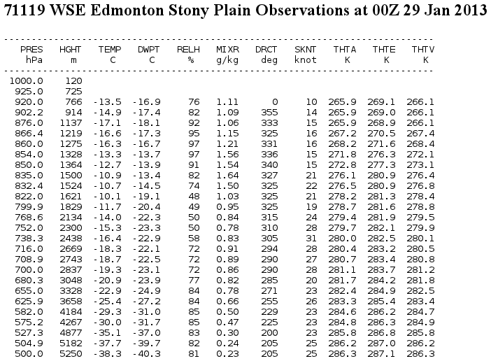
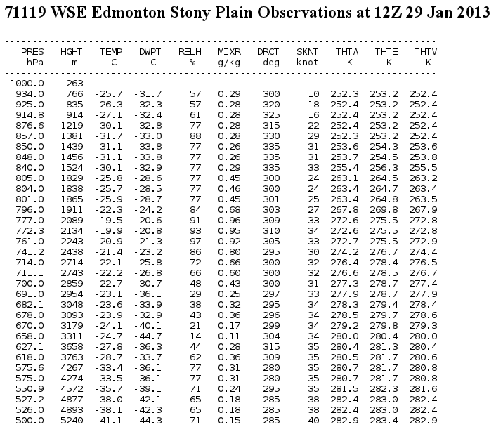
- Tues 29 Jan. Exercise -- follow-up on 120-hr forecast from last Thursday (here is the needed 850 hPa analysis for 00Z today).
Answers: Taking the 850 hPa wind speed as 10 m s-1 (the radiosonde value), JDW gets -1.9 K hr-1 for the advective cooling rate, implying about 23oC cooling over 12 hours. However this is very much an approximation, for one's evaluation of the temperature gradient is subjective. The observed overnight change in temperature (00Z to 12Z Jan. 29) at the 850 hPa level was about 18oC (-13oC to -31oC), as is evident by comparing the 850 hPa analyses (00Z and 12Z) or the soundings (00Z and 12Z). The observed temperature change at the surface was about 12oC.
- Thurs 24 Jan. Developing cyclone - example (from prog). Derivation of the continuity equation. Velocity divergence (3D & 2D). Today's exercise (10:20-10:50): on the basis of available progs (e.g. GEM-glbl and NCEP's GFS), give your weather forecast for central Alberta for the period 12Z Tues 29 - 12Z Wed 30 Jan. Jot down your qualitative prediction for the weather elements (i.e. temperature, sky condition, precip, wind speed); and compare the forecast 1000-500 thickness with the present value. Any major uncertainties should be acknowledged. (Please submit at end of class).
Here are (some of) the available NWP charts, along with follow-up (verification).
- Tues 22 Jan. Orientation to Assignment 2: contingency tables, and the Heidke Skill Score. Complete exercises of previous class (excepting that which has been struck out). Further exercises.
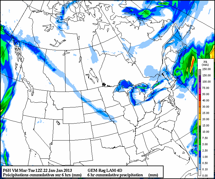
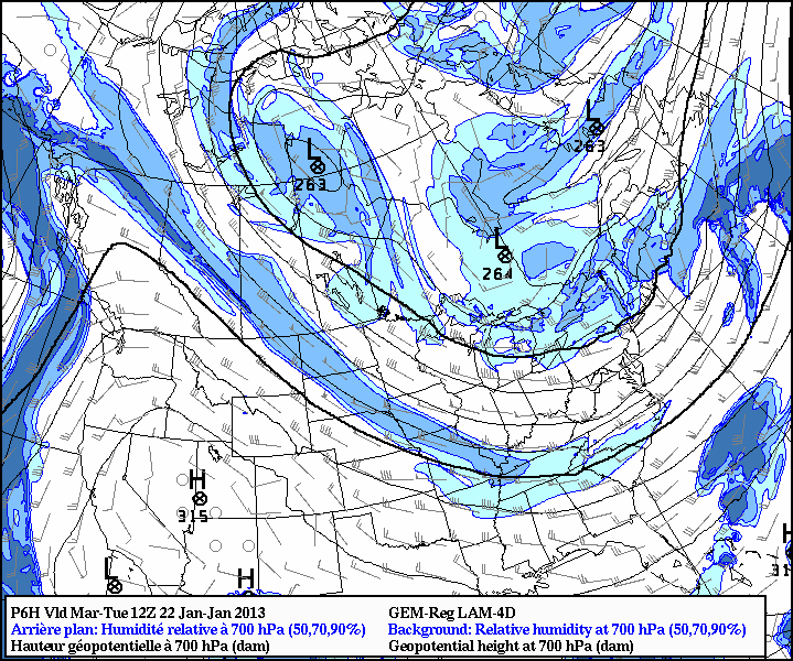
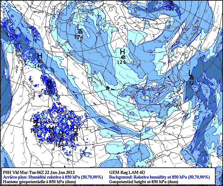
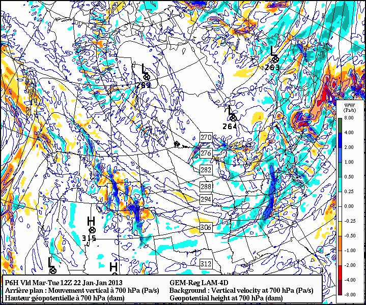
GEM panels (from GEM-reg run initialized 06Z Tues 22 Jan.) relevant to today's exercise:
In short, GEM's prediction - though (apparently) incorrect - is consistent with the patterns of precipitable water and of humidity in the lower to middle tropsphere. Patchy weak updrafts (seen at 700 hPa) also fit (loosely) with the forecast pattern of prediction.
- Thurs 17 Jan. Review of vector notation; the grad operator; the horizontal momentum equation. The geostrophic wind law in terms of the pressure gradient and in terms of the height gradient. The natural coordinate system. Thermal wind and thermal wind balance. Connection between directional wind shear and thermal advection. Exercises & today's weather situation.
Answers: The geostrophic wind speed Vg≈29 m s-1. The computed rate of temperature advection at Pickle Lake is approximately -1.5 K hr-1 (be sure to compute the distance between isotherms along a line parallel to the wind vector).
- Tues 15 Jan. Review the families of curves on the Skew-T diagram. Completion of exercises from previous class. Weather situation (following up on the 1-week forecast, valid today, from last Tuesday). If time permits: computing the geostrophic wind speed
- Thurs 10 Jan. Today's local weather situation and outlook. The hypsometric equation in relation to Assignment 1 (a derivation starting from the hydrostatic equation). Exercises (and maps relating to the weather situation). We reviewed some elements relating to weatehr maps (the 850 and 700 hPa "mandatory levels" and their heights above sea-level; the Geostrophic relationship betwen wind speed & direction, and the height contours). Regarding the morning's specific weather situation, we noted the weak temperature gradient at the 850 hPa level and inferred that further cooling will not be rapid; we observed the cold front now over Saskatchewan, correlating it to the forecasters' discussion.
Answers: ρ=1.23 kg m-3. RH=87% (agreeing with value tabulated). Δz=(766-723)=43 m, which implies (using the computed value for ρ) that |Δp|=1.23 x 9.81 x 43 = 519 Pa, for a surface pressure at YEG of 925+5.19=930.19 hPa. The potential temperature θ=(273.15-35.1) x (1000/500)^(287/1000)=290.4 K = 17.3oC.
- Tues 8 Jan. Introduction, scope, aims and structure of the course, evaluation etc. Familiarization with web weather resources. Exercise regarding this morning's weather, and outlook.